Cluster analysis

- Have a working knowledge of the ways in which similarity between cases can be quantified (e.g. single linkage, complete linkage and average linkage).
- Be able to produce and interpret dendrograms produced by SPSS.
- Know that different methods of clustering will produce different cluster structures.
What is Cluster Analysis?
We have already seen that we can use Factor Analysis to group variables according to shared variance. In factor analysis, we take several variables, examine how much variance these variables share, and how much is unique and then ‘cluster’ variables together that share the same variables. In short, we cluster together variables that look as though they explain the same variance. The example in my textbooks (Field 2025, 2024) measuring attitudes to SPSS or R, and the result of the factor analysis was to isolate groups of questions that seem to share their variance in order to isolate different dimensions of SPSS or R anxiety.
Why am I talking about factor analysis? Well, in essence, cluster analysis is a similar technique except that rather than trying to group together variables, we are interested in grouping cases Usually, in psychology at any rate, this means that we are interested in clustering groups of people. So, in a sense it’s the opposite of factor analysis: instead of forming groups of variables based on several people’s responses to those variables, we instead group people based on their responses to several variables.
So, as an example if we measured anal-retentiveness, number of friends and social skills we might find two distinct clusters of people: statistics lecturers (who score high on anal-retentiveness and low on number of friends and social skills) and students (who score low on anal-retentiveness and high on number of friends and social skills).
Cluster Analysis is a way of grouping cases of data based on the similarity of responses to several variables.
How Does Cluster Analysis Work?
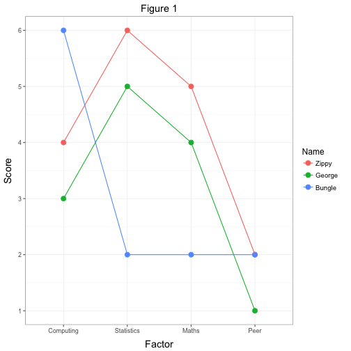
Imagine a simple scenario in which we’d measured Zippy, Bungle and George’s (Figure 1) scores on my (fictional) SPSS Anxiety Questionnaire, SAQ (Field 2024).
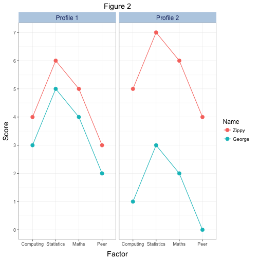
This questionnaire resulted in four factors: computing anxiety, statistics anxiety, maths anxiety and anxiety relating to evaluation from peers. Our three people fill out the questionnaire and from our factor analysis we get factor scores for each of these four components. As a simple measure of the similarity of their scores we could plot a line showing the relationship between their scores (Figure 2)
Looking at Figure 2 it’s pretty clear that Zippy and George have a very similar pattern of responses across the four factors (in fact their lines are parallel, indicating that the relative difference in their scores across factors is the same). Bungle, however, has a very different set of responses. He has a very similar score to Zippy and George for the ‘peer evaluation’ factor but for the remaining three factors his scores are very different to the other two. Therefore, we could cluster Zippy and George together based on the fact that the profile of their responses is very similar.
How is Similarity Measured?
Obviously, looking at graphs of responses if a very subjective way to establish whether two people have similar responses across variables. In addition, in situations in which we have hundreds of people and lots of variables, the graphs of responses that we plot would become very cumbersome and almost impossible to interpret. Therefore, we need some objective way to measure the degree of similarity between people’s scores across a number of variables. There are two types of measure: similarity coefficients and dissimilarity coefficients. Can you think of a measure of similarity of two variables that you’ve come across before (numerous times) that could be adapted to measure the similarity of people?
Correlation Coefficient, r
The correlation coefficient is a measure of similarity between two variables (it tells us whether as one variable changes the other changes by a similar amount). In theory, we could apply the correlation coefficient to two people rather than two variables to see whether the pattern of responses for one person is the same as the other. The correlation coefficient is a standardised measure and so it has the advantage that it is unaffected by dispersion differences across variables (in plain English this means that if the variables across which we’re comparing people are measured in different units the correlation coefficient will not be affected). However, there is a problem with using a simple correlation coefficient to compare people across variables: it ignores information about the elevation of scores. Therefore, although the correlation coefficient tells us whether the pattern of responses between people are similar, it doesn’t tell us anything about the distance between two people’s profiles.
Figure 3 shows two examples of responses across the factors of the SAQ. In both diagrams the two people (Zippy and George) have similar profiles (the lines are parallel). Therefore, the resulting correlation coefficient for the two graphs would be identical (in fact, you’d get a perfect correlation of 1). However, the distance between the two profiles is much greater in the second graph (the elevation is higher). Therefore, it might be reasonable to conclude that the people in the first graph are more similar than the two in the second graph, yet the correlation coefficient is the same. As such, the correlation coefficient misses important information.
Euclidean Distance, \(d\)
An alternative measure is the Euclidean distance. Euclidean distance is the geometric distance between two objects (or cases). Therefore, if we were to call George subject i and Zippy subject j, then we could express their Euclidean distance in terms of the following equation:
\[ d_{ij} = \sqrt{\sum_{k = 1}^{p}{(x_{ik} - x_{jk})^2}} \]
This equation means that we can discover the distance between Zippy and George by taking their scores on a variable, k, and calculating the difference. Now, for some variables Zippy will have a bigger score than George and for other variables George will have a bigger score than Zippy. Therefore, some differences will be positive and some negative. Eventually we want to add up the differences across a number of variables, and so if we have positive and negative difference they might cancel out. To avoid this problem, we simply square each difference before adding them up. OK, so far we’ve got Zippy and George’s scores for variable k and we’ve calculated the difference and squared it. All we do now is move onto the next variable and do the same. When we’ve done the same for every variable we add all of the differences up (it’s just like calculating the variance really). When we’ve added all of the squared differences we take the square root (because by squaring the differences we’ve changed the units of measurement to units2 and so by taking the square root we revert back to the original units of measurement).
In reality, the average Euclidean distance is used (so after summing the squared differences we simply divide by the number of variables) because it allows for missing data. With Euclidean distances the smaller the distance, the more similar the cases. However, this measure is heavily affected by variables with large size or dispersion differences. So, if cases are being compared across variables that have very different variances (i.e. some variables are more spread out than others) then the Euclidean distances will be inaccurate. As such it is important to standardise scores before proceeding with the analysis. Standardising scores is especially important if variables have been measured on different scales.
Creating the Clusters
Once we have a measure of similarity between cases, we can think about ways in which we can group cases based on their similarity. There are several ways to group cases based on their similarity coefficients. Most of these methods work in a hierarchical way. The principle behind each method is similar in that it begins with all cases being treated as a cluster in its own right. Clusters are then merged based on a criterion specific to the method chosen. So, in all methods we begin with as many clusters as there are cases and end up with just one cluster containing all cases. By inspecting the progression of cluster merging it is possible to isolate clusters of cases with high similarity.
Single Linkage or SLINK (Nearest Neighbour)
This is the simplest method and so is a good starting point for understanding the basic principles of how clusters are formed (and the hierarchical nature of the process). The basic idea is as follows:
- Each case begins as a cluster.
- Find the two most similar cases/clusters (e.g. A & B) by looking at the similarity coefficients between pairs of cases (e.g. the correlations or Euclidean distances). The cases/clusters with the highest similarity are merged to form the nucleus of a larger cluster.
- The next case/cluster to be merged with this larger cluster is the one with the highest similarity coefficient to either A or B.
- The next case merged is the one with the highest similarity to A, B or C, and so on.
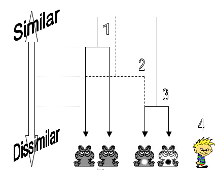
Figure 4 shows how the simple linkage method works. If we measured 5 animals on their physical characteristics (colour, number of legs, eyes etc.) and wanted to cluster these animals based on these characteristics we would start with the two most similar animals. First, imagine the similarity coefficient as a vertical scale ranging from low similarity to high. In the simple linkage method, we begin with the two most similar cases. We have two animals that are very similar indeed (in fact they look identical). Their similarity coefficient is therefore high. A fork that splits at the point on the vertical scale representing the similarity coefficient represents the similarity between these animals. So, because the similarity is high the points of the fork are very long. This fork is (1) in the diagram.
Having found the first two cases for our cluster we look around for other cases. In this simple case there are three animals left. The animal chosen to next be part of the cluster is the one most similar to either one of the animals already in the cluster. In this case, there is an animal that is similar in all respects except that it has a white belly. The other two cases are less similar (because one is a completely different colour and the other is human!). The similarity coefficient of the chosen animal is slightly lower than for the first two (because it has a white belly) and so the fork (represented by a dotted line) divides at a lower point along the vertical scale. This stage is (2) in the diagram.
Having added to the cluster we again look at the remaining cases and assess their similarity to any of the three animals already in the cluster. There is one animal that is fairly similar to the animal just added to the cluster. Although it is a different colour, it has the same distinctive pattern on its belly. Therefore, this animal is added to the cluster on the basis of its similarity to the third animal in the cluster (even though it is relatively dissimilar to the other two animals). This is (3) in the diagram.
Finally, there is one animal left (the human) who is dissimilar to all of the animals in the cluster, therefore, he will eventually be merged into the cluster, but his similarity score will be very low. There are several important points here. The first is that the process is hierarchical. Therefore, the results we get will very much depend on the two cases that we chose as our starting point. Second, cases in a cluster need only resemble one other case in the cluster, therefore, over a series of selections a great deal of dissimilarity between cases can be introduced. Finally, the diagram we’ve drawn connecting the cases is known as a dendrogram (or tree diagram). The output of a cluster analysis is in the form of this kind of diagram.
Complete Linkage or CLINK (Furthest Neighbour)
A variation on the simple linkage method is known as complete linkage (or the furthest neighbour). This method is the logical opposite to simple linkage. To begin with the procedure is the same as simple linkage in that initially we look for the two cases with the highest similarity (in terms of their correlation or average Euclidean distance). These two cases (A & B) form the nucleus of the cluster. The second step is where the difference in method is apparent. Rather than look for a new case that is similar to either A or B we look for a case that has the highest similarity score to both A and B. The case © with the highest similarity to both A and B is added to the cluster. The next case to be added to the cluster is the one with the highest similarity to A, B and C. This method reduces dissimilarity within a cluster because it is based on overall similarity to members of the cluster (rather than similarity to a single member of a cluster). However, the results will still depend very much on which two cases you take as your starting point.
Average (Between-Group) Linkage
This method is another variation on simple linkage. Again, we begin by finding the two most similar cases (based on their correlation or average Euclidean distance). These two cases (A & B) form the nucleus of the cluster. At this stage the average similarity within the cluster is calculated. To determine which case © is added to the cluster we compare the similarity of each remaining cases to the average similarity of the cluster. The next case to be added to the cluster is the one with the highest similarity to the average similarity value for the cluster. Once this third case has been added, the average similarity within the cluster is re-calculated. The next case (D) to be added to the cluster is the one most similar to this new value of the average similarity.
Ward’s Method
The linkage methods are all based on a similar principle: there is a chain of similarity leading to whether or not a case is added to a cluster. The rules governing this chain differ from one linkage method to another. A different approach is Ward’s method, which is considerably more complex than the simple linkage method. The aim in Ward’s method is to join cases into clusters such that the variance within a cluster is minimised. To do this, each case begins as its own cluster. Clusters are then merged in such a way as to reduce the variability within a cluster.To be more precise, two clusters are merged if this merger results in the minimum increase in the error sum of squares. Basically, this means that at each stage the average similarity of the cluster is measured. The difference between each cases within a cluster and that average similarity is calculated and squared (just like calculating a standard deviation). The sum of squared deviations is used as a measure of error within a cluster. A cases is selected to enter the cluster if it is the case whose inclusion in the cluster produces the least increase in the error (as measured by the sum of squared deviations).
Limitations of Cluster Analysis
There are several things to be aware of when conducting cluster analysis:
- The different methods of clustering usually give very different results. This occurs because of the different criterion for merging clusters (including cases). It is important to think carefully about which method is best for what you are interested in looking at.
- With the exception of simple linkage, the results will be affected by the way in which the variables are ordered.
- The analysis is not stable when cases are dropped: this occurs because selection of a case (or merger of clusters) depends on similarity of one case to the cluster. Dropping one case can drastically affect the course in which the analysis progresses.
- The hierarchical nature of the analysis means that early ‘bad judgements’ cannot be rectified.
Cluster Analysis using IBM SPSS Statistics
We’ll stick to a basic example. Imagine we wanted to look at clusters of cases referred for psychiatric treatment. We measured each subject on four questionnaires: Spielberger Trait Anxiety Inventory (STAI), the Beck Depression Inventory (BDI), a measure of Intrusive Thoughts and Rumination (IT) and a measure of Impulsive Thoughts and Actions (Impulse). The rationale behind this analysis is that people with the same disorder should report a similar pattern of scores across the measures (so the profiles of their responses should be similar). To check the analysis, we asked 2 trained psychologists to agree a diagnosis based on the DSM-IV. These data are in Figure 5 and in the file diagnosis.sav.

The first thing to note is that like factor analysis and regression, data for each variable is placed in a separate column. Therefore, each row of the Data Editor represents a single subject’s data.
Running the Analysis
Figure 6 shows the main dialogue box for running cluster analysis. This dialogue box is obtained using the menu path Analyze > Classify > Hierarchical Cluster. Select the four diagnostic questionnaires from the list on the left-hand side and drag them to the box labelled Variables. The variable DSM is included in the data editor merely as a way of helping demonstrate what the output from a cluster analysis means, therefore, we do not need to include it in the analysis.
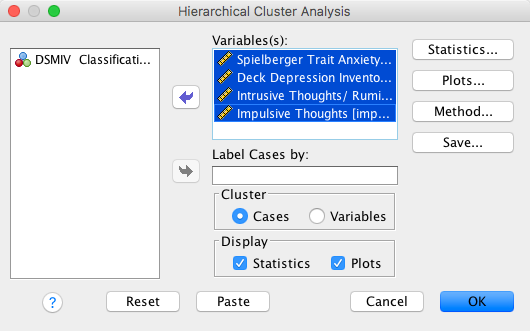
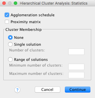
If you click on Statistics in the main dialog box then another dialog box appears (see Figure 7). The main use of this dialog box is in specifying a set number of clusters. By default, SPSS will merge all cases into a single cluster and it is down to the researcher to inspect the output to determine substantive sub-clusters. However, if you have a hypothesis about how many clusters should emerge, then you can tell SPSS to create a set number of clusters, or to create a number of clusters within a range. For this example, leave the default options as they are and proceed back to the main dialog box by clicking Continue.
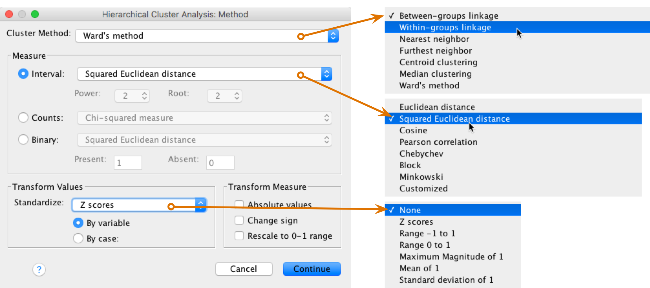
Click on Method … to access the dialog box in Figure 8. You use this dialog box to choose the method of creating clusters (some of which were described above). By default SPSS uses between-groups linkage (or average linkage) methods. However, several other options are available (e.g. nearest neighbour, furthest neighbour and Ward’s method). Each method can be selected by clicking on the down arrow where it says Cluster Method. For this analysis, I suggest choosing Ward’s method, but as practise I suggest coming back and trying some different methods: you’ll find you get very different results!
Underneath the method selection, there are a series of options depending on whether you’re analysing interval data (as we are here), frequency data (counts) or binary data (dichotomous variables with only two possible responses). Each of these types of data has an associated set of measures of similarity. Earlier I described Euclidean distances and the correlation coefficient. By default, SPSS uses Euclidean distances (which is a good option to use). However, you cans elect a different measure of similarity if required (see Romesburg 1984; Everitt et al. 2011 for detail of the possible methods).
Finally, at the bottom of the dialog box is the option to standardise our data. I mentioned earlier that standardising data is a good idea (especially because some measures of similarity are sensitive to differences in the variance of variables) therefore I recommend this option. There are a number of ways in which data can be standardized but the most easily understood is to convert to a z-score. I suggest this option. It is possible to standardise either by variable, or across a particular case. When clustering cases (as we’re doing here, known as Q-analysis) we must standardise the variables. If we were trying to cluster variables (R-analysis) then we would need to standardise across cases. So, for this example, select z-scores for variables and proceed by clicking Continue.
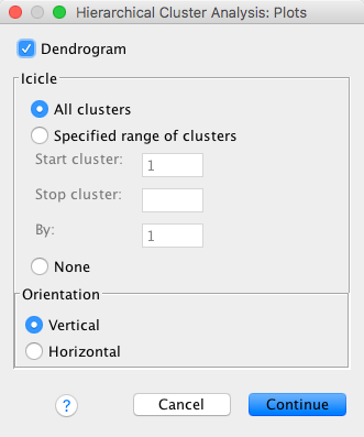
Once back in the main dialog box, you can select the plots dialog box by clicking Plots … (Figure 9). There are two types of diagram that you can ask for from a cluster analysis. The default option is an icicle plot, but the most useful for interpretation purposes is the dendrogram. The dendrogram shows us the forks (or links) between cases and its structure gives us clues as to which cases form coherent clusters. Therefore, it’s essential to request this option. Once this option is selected, click on Continue.
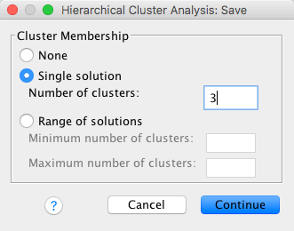
Once back in the main dialog box, you can select the save dialog box by clicking Save …. This dialog box allows us to save a new variable into the data editor that contains a coding value representing membership to a cluster. As such, we can use this variable to tell us which cases fall into the same clusters. By default, SPSS does not create this variable. In this example, we’re expecting three clusters of people based on the DSM-IV classifications (GAD, depression and OCD) so we could select Single solution and then type 3 in the blank space (see Figure 10).
In reality, what we would normally do is to run the cluster analysis without selecting this option and then inspect the resulting dendrogram to establish how many substantive clusters lie within the data. Having done this, we could re-run the analysis, requesting that SPSS save coding values for the number of clusters that we identified.
Output from SPSS: The Dendrogram
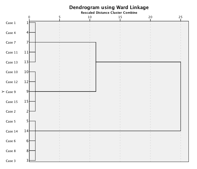
The main part of the output from SPSS is the dendrogram (although ironically this graph appears only if a special option is selected). The dendrogram for the diagnosis data is presented in Figure 11.
As explained earlier, cluster analysis works upwards to place every case into a single cluster. Therefore, we end up with a single fork that subdivides at lower levels of similarity. For these data, the fork first splits to separate cases 1, 4, 7, 11, 13, 10, 12, 9, 15, & 2 from cases 5, 14, 6, 8, & 3. In actual fact, if you look at the DSM-IV classification for these subjects, this first separation has divided up GAD and Depression from OCD. This is likely to have occurred because both GAD and Depression patients have low scores on intrusive thoughts and impulsive thoughts and actions whereas those with OCD score highly on both measures. The second major division is to split one branch of this first fork into two further clusters. This division separates cases 1, 4, 7, 11 & 13 from 10, 12, 9, 15, & 2.
Looking at the DSM classification this second split has separated GAD from Depression. In short, the final analysis has revealed 3 major clusters, which seem to be related to the classifications arising from DSM. As such, we can argue that using the STAI, BDI, IT and Impulse as diagnostic measures is an accurate way to classify these three groups of patients (and possibly less time consuming than a full DSM-IV diagnosis). Obviously these data are rather simplistic and have resulted in a very uncomplicated solution. In reality there is a lot subjectivity involved in deciding which clusters are substantive.
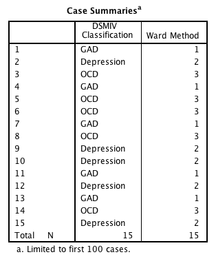
Having eyeballed the dendrogram and decided how many clusters are present it is possible to re-run the analysis asking SPSS to save a new variable in which cluster codes are assigned to cases (with the researcher specifying the number of clusters in the data). For these data, we saw three clear clusters and so we could re-run the analysis asking for cluster group codings for three clusters (in fact, I told you to do this as part of the original analysis). Figure 12 shows the resulting codes for each case in this analysis. It’s pretty clear that these codes map exactly onto the DSM-IV classifications. Although this example is very simplistic it shows you how useful cluster analysis can be in developing and validating diagnostic tools, or in establishing natural clusters of symptoms for certain disorders.
Further reading
Exercise
Cluster analysis can also be used to look at similarity across variables (rather than cases). The data in the file clusterdisgust.sav are from Sarah Marzillier’s D.Phil1. research and show different aspects of disgust rated by many different people (each column represents some aspect of disgust — the variable labels show what each column represents). We could run a cluster analysis to see which aspects of disgust cluster together based on the similarity of people’s responses to them. Run a cluster analysis on these data but select Cluster Variables in the initial dialog box (see Figure 4). Which aspects of disgust cluster together?
1 Thanks to Sarah Marzillier for letting me use her data as an example